
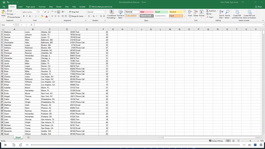
This quick tip is another Excel one. If the your data has headers, you can quickly turn those headers into filters. Even if your data does not have headers, you can quickly add them. Here’s how:
- Select the entire row with your headers (typically the first row)
- Select the Data Tab
- In the Ribbon, click on Filter
- Excel will automatically create filters, using unique data in each column as options
- Click on the triangle icon to the right of the header you want to filter
- Click on the checkbox to the left of Select All to deselect all of the options
- Then, go down the list and select the options you want to filter by
- Click on OK
- Excel will automatically filter the data based on your criteria. If needed, multiple filters can be used at once
- To reset the filter, click on the symbol to the right of the header with the filter
- In the menu that appears, click on Clear Filter from “Header Name”
Click on the image below to view our tutorial video:
For more tutorials on Excel and other Microsoft Office products, visit the Microsoft Office Support Wiki Page.